Tutorial 7 — Van Gurp–Palmen and Cole–Cole plots - hermes-rheo

hermes_rheo.visualization provides two diagnostic plots for oscillatory data. Both take an experiment set and read the variable names and units from its datasets.

Function	x	y
`plot_vgp`	$\lvert G^*\rvert = \sqrt{G'^2 + G''^2}$	$\tan\delta = G''/G'$
`plot_cole_cole`	$G'$	$G''$

Both plots eliminate frequency and temperature as explicit variables. In the van Gurp–Palmen (vGP) plot (van Gurp and Palmen, 1998), a horizontal shift $\omega \to a_T\,\omega$ leaves each pair $\lvert G^*\rvert$ , $\tan\delta$ unchanged, so data measured at different temperatures collapse onto one curve if time–temperature superposition holds (Tutorial 4). Scatter between isotherms therefore indicates thermorheological complexity, for example in blends, long-chain branched or phase-separated materials. The curve shape is also a fingerprint of molecular structure: $\tan\delta$ grows without bound in the terminal (viscous) region, and a minimum marks the rubbery plateau.

The Cole–Cole plot (Cole and Cole, 1941), originally used for dielectric relaxation, plots $G''$ against $G'$ and is used in the same way. A single Maxwell mode gives a semicircle on linear axes; broader relaxation spectra flatten and skew the curve.

import warnings
from pathlib import Path

import matplotlib.pyplot as plt

from hermes_rheo import read_file
from hermes_rheo.file_readers.trios_rheo_txt import TriosRheoReader
from hermes_rheo.visualization import plot_cole_cole, plot_vgp, use_science_style

use_science_style()
warnings.filterwarnings("ignore")  # scikit-learn / SciPy convergence notices
DATA = Path("tutorial_data")

def load(name):
    return read_file(DATA / name, file_reader=TriosRheoReader, create_composite_datasets=True)

Frequency sweeps¶

Conventional frequency sweeps at several temperatures (the data of Tutorial 4), one curve per isotherm.

sweep = load("aresg2_trios_frequency_sweep_tts.txt")
fig, axes = plt.subplots(1, 2, figsize=(10, 4))
plot_vgp(sweep, ax=axes[0])
plot_cole_cole(sweep, ax=axes[1])
plt.show()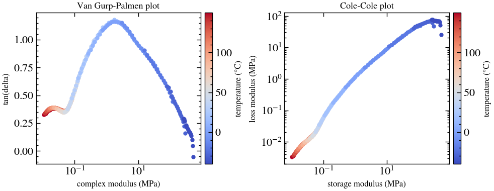

Temperature-ramped chirps (TORCh)¶

In a Thermally Optimised Ramped Chirp (TORCh) experiment, OWChirps are applied continuously during a temperature ramp (Vadillo et al., 2026). This file already contains the frequency-domain moduli of every chirp, so it is plotted directly. If the chirps were recorded with the TRIOS Arbitrary Wave procedure, the file holds only time-domain stress and strain signals; apply OWChirpAnalysis first (Tutorial 3), e.g. plot_vgp(OWChirpAnalysis()(experiment)).

torch = load("dhr30_trios_torch.txt")
fig, axes = plt.subplots(1, 2, figsize=(10, 4))
plot_vgp(torch, ax=axes[0], marker="o", markersize=3)
plot_cole_cole(torch, ax=axes[1], marker="o", markersize=3)
plt.show()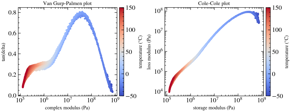

Both functions draw onto an existing axes (ax) and colour each measurement by temperature (colormap), with a legend for a few curves or a colour bar for many (legend). They plot any pair of data arrays (x_name, y_name), can save the figure (save), and forward extra keywords to ax.plot. See the visualization API for these options and the other plotting helpers.

References¶

van Gurp, M. and Palmen, J., Time-temperature superposition for polymeric blends, Rheology Bulletin 67, 5–8 (1998).
Cole, K. S. and Cole, R. H., Dispersion and Absorption in Dielectrics — I. Alternating Current Characteristics, Journal of Chemical Physics 9, 341–351 (1941). DOI: 10.1063/1.1750906.
Vadillo, D. C., Perego, A. et al., TORCh: Thermally Optimised Ramped Chirp for time-temperature spectroscopy of polymers, Macromolecules (2026). DOI: Vadillo et al. (2026).

References¶

Vadillo, D. C., Perego, A., Whitcomb, K., Behling, R. E., Gill, A. M., Das, M., & McKinley FRS, G. H. (2026). TORCh: Thermally Optimized Ramped Chirps for the Efficient Generation of Rheological Master Curves. Macromolecules, 59(12), 6893–6905. 10.1021/acs.macromol.6c00679