Tutorial 10 — Recovery rheology - hermes-rheo

Recovery rheology splits the total shear strain of a viscoelastic material into a recoverable (elastic) part and an unrecoverable (viscous or plastic) part (Lee et al., 2019),

\gamma_\mathrm{tot} = \gamma_\mathrm{rec} + \gamma_\mathrm{unrec}.

(1)

The recoverable strain is measured directly: the imposed deformation is interrupted, the stress is set to zero, and the strain that returns is recorded. Each component then defines its own material function, the recoverable modulus $G_\mathrm{rec} = \sigma/\gamma_\mathrm{rec}$ and the flow viscosity $\eta_\mathrm{flow} = \sigma/\dot\gamma_\mathrm{unrec}$ (Singh et al., 2021). This separates solid-like from fluid-like contributions that conventional moduli mix, for example across a yield transition (Donley et al., 2020).

RecoveryRheology analyses Anton Paar RheoCompass exports with two protocols:

method="oscillatory" (oscillatory recovery): oscillations interrupted by zero-stress recovery steps. Forward and reverse runs with opposite strain amplitude are averaged as $(A - B)/2$ , which keeps the response that is odd in strain and cancels drift that does not change sign.
method="step" (step-function recovery): strain- or stress-controlled deformation steps of increasing duration, each followed by a zero-stress recovery step.

All recovery data in this tutorial are full resolution.

from pathlib import Path

import matplotlib.pyplot as plt

from hermes_rheo import read_file
from hermes_rheo.file_readers.rheo_compass_csv import RheoCompassReader
from hermes_rheo.transforms.recovery_rheology import (
    RecoveryRheology,
    batch_oscillatory_recovery,
    plot_decomposed_moduli,
)
from hermes_rheo.visualization import use_science_style

use_science_style()
DATA = Path("tutorial_data")

Oscillatory recovery¶

The Fourier component of the averaged stress at the test frequency $\omega$ gives the conventional $G'$ and $G''$ . The transform then reconstructs a full period of the strain, recoverable strain and stress, and computes cycle-averaged energies for each strain component $x \in \{\mathrm{tot}, \mathrm{rec}, \mathrm{unrec}\}$ :

G'_x = \frac{2\,\langle \gamma_x\,\sigma \rangle}{\gamma_0^2}, \qquad G''_x = \frac{2\,\langle \dot\gamma_x\,\sigma \rangle}{(\omega\,\gamma_0)^2},

(2)

where $\gamma_0$ is the total-strain amplitude. $G'_\mathrm{solid} = G'_\mathrm{rec}$ is the energy stored elastically, $G''_\mathrm{solid} = G''_\mathrm{rec}$ the energy dissipated by recoverable deformation, and $G''_\mathrm{fluid} = G''_\mathrm{unrec}$ the energy dissipated by flow. Supply the known omega (rad/s); otherwise it is estimated from the data.

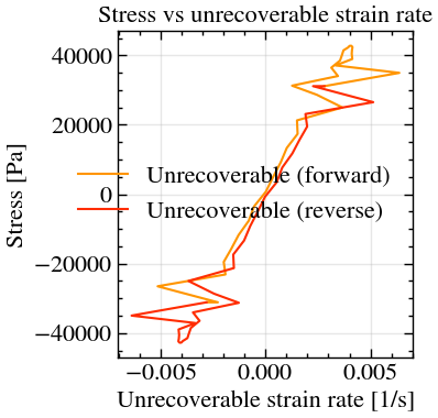
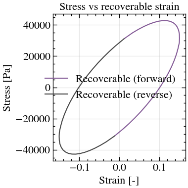
Lissajous figures plot the stress against total strain, recoverable strain and unrecoverable strain rate. A stress– $\gamma_\mathrm{rec}$ loop that collapses to a straight line indicates purely elastic recovery, while the stress– $\dot\gamma_\mathrm{unrec}$ loop shows the fluid contribution.

oscillatory = read_file(DATA / "mcr702e_rheocompass_recovery_oscillatory.csv",
                        file_reader=RheoCompassReader, create_composite_dataset=True)

oscillatory_recovery = RecoveryRheology(method="oscillatory", omega=0.316)(oscillatory).result
figures, axes = oscillatory_recovery.plot_lissajous(figsize=(4, 4))
plt.show()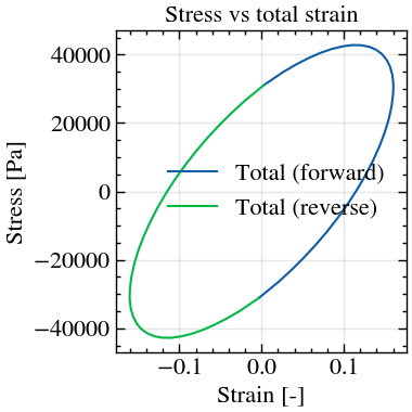

Amplitude series¶

batch_oscillatory_recovery applies the analysis to every file in a folder; here, one polymer melt at the same temperature and $\omega = 0.316$ rad/s for strain amplitudes from 1 % to 631 %. In the linear regime the decomposed moduli are constant and $G'_\mathrm{solid}$ dominates. At large amplitudes, $G'_\mathrm{solid}$ decreases while $G''_\mathrm{fluid}$ grows, showing the transition from recoverable deformation to flow. Pass export_dir= to also write the per-file Excel results and Lissajous figures.

amplitude_series = batch_oscillatory_recovery(DATA / "recovery_series", n_osc=2, diff_state=4, k_step=1)
fig, ax = plot_decomposed_moduli(amplitude_series, x_axis="strain")
plt.show()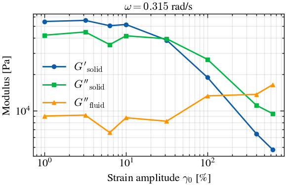

Step-function recovery¶

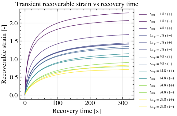
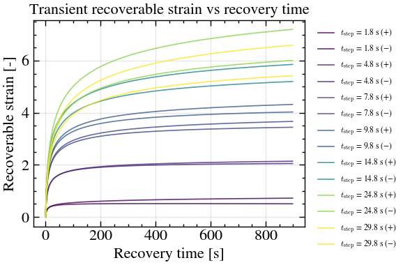
Each deformation step is followed by recovery at zero stress. The strain left after recovery is $\gamma_\mathrm{unrec}$ , and the recovered strain is

\gamma_\mathrm{rec}(t_\mathrm{r}) = \gamma_\mathrm{tot}(t_\mathrm{exp}) - \gamma(t_\mathrm{r}),

(3)

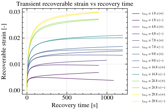
where $t_\mathrm{exp}$ is the end of the deformation and $t_\mathrm{r}$ the recovery time. Increasing the step duration maps how the recoverable and unrecoverable strains build up during the deformation. plot_step_results shows the three strains against experimental time; plot_transient shows the recovered strain against recovery time for each step. The same analysis applies to any deformation step; the three examples below use step strain, creep and start-up shear.

Step strain¶

A strain of 2000 % ( $\gamma_\mathrm{tot} = 20$ ) is held for increasing durations at 100 °C. The total strain is fixed, so the analysis shows how it is partitioned: as the stress relaxes during longer holds, more of the imposed strain becomes unrecoverable and less is recovered.

step_strain_data = read_file(DATA / "mcr702e_rheocompass_step_strain_recovery.csv",
                            file_reader=RheoCompassReader, create_composite_dataset=True)

step_strain_recovery = RecoveryRheology(method="step")(step_strain_data).result
fig, ax = step_strain_recovery.plot_step_results(figsize=(6, 4))
plt.show()
fig, ax = step_strain_recovery.plot_transient(figsize=(6, 4), logx=False)
plt.show()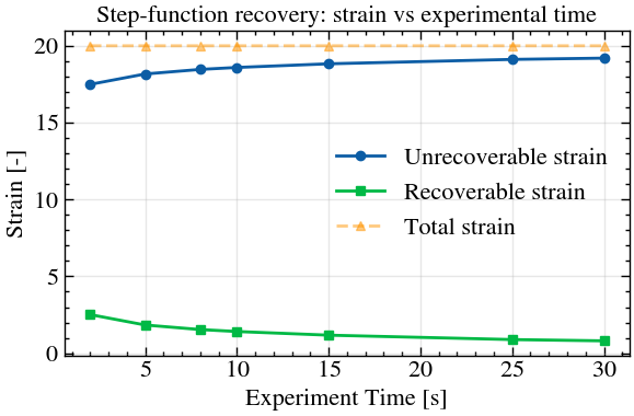

Creep¶

A constant stress of 100 Pa is applied for increasing durations at 70 °C. The total strain grows with the creep time; at this stress most of it is recovered, and the unrecoverable strain, the flow contribution, builds up slowly.

creep_data = read_file(DATA / "mcr702e_rheocompass_creep_recovery.csv",
                      file_reader=RheoCompassReader, create_composite_dataset=True)

creep_recovery = RecoveryRheology(method="step")(creep_data).result
fig, ax = creep_recovery.plot_step_results(figsize=(6, 4))
plt.show()
fig, ax = creep_recovery.plot_transient(figsize=(6, 4), logx=False)
plt.show()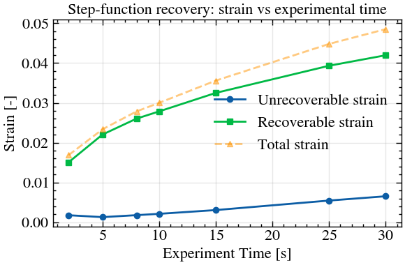

Start-up shear¶

A constant shear rate of 1 s $^{-1}$ is applied for increasing durations at 70 °C, so the total strain grows linearly with time. The recoverable strain saturates as the material approaches steady flow, after which the additional strain is unrecoverable.

startup_shear_data = read_file(DATA / "mcr702e_rheocompass_startup_shear_recovery.csv",
                              file_reader=RheoCompassReader, create_composite_dataset=True)

startup_shear_recovery = RecoveryRheology(method="step")(startup_shear_data).result
fig, ax = startup_shear_recovery.plot_step_results(figsize=(6, 4))
plt.show()
fig, ax = startup_shear_recovery.plot_transient(figsize=(6, 4), logx=False)
plt.show()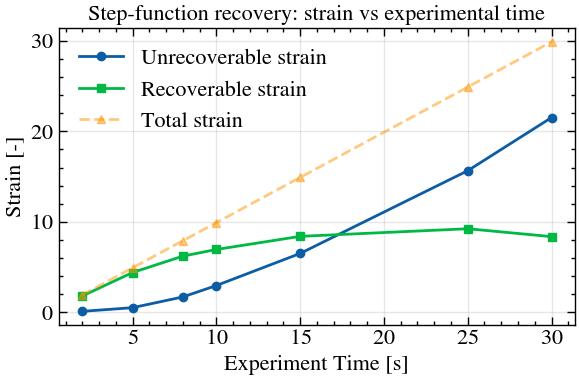

Both result objects export the transient data and moduli with to_excel(path).

References¶

Lee, J. C.-W., Weigandt, K. M., Kelley, E. G. and Rogers, S. A., Structure–Property Relationships via Recovery Rheology in Viscoelastic Materials, Physical Review Letters 122, 248003 (2019). DOI: Lee et al. (2019).
Donley, G. J., Singh, P. K., Shetty, A. and Rogers, S. A., Elucidating the G″ overshoot in soft materials with a yield transition via a time-resolved experimental strain decomposition, Proceedings of the National Academy of Sciences 117, 21945–21952 (2020). DOI: Donley et al. (2020).
Singh, P. K., Lee, J. C.-W., Patankar, K. A. and Rogers, S. A., Revisiting the basis of transient rheological material functions: Insights from recoverable strain measurements, Journal of Rheology 65, 129–144 (2021). DOI: 10.1122/8.0000154.
Shi, J. and Rogers, S. A., The benefits of a formalism built on recovery: Theory, experiments, and modeling, Journal of Non-Newtonian Fluid Mechanics 321, 105113 (2023). DOI: 10.1016/j.jnnfm.2023.105113.

References¶

Lee, J. C.-W., Weigandt, K. M., Kelley, E. G., & Rogers, S. A. (2019). Structure-Property Relationships via Recovery Rheology in Viscoelastic Materials. Physical Review Letters, 122(24). 10.1103/physrevlett.122.248003
Donley, G. J., Singh, P. K., Shetty, A., & Rogers, S. A. (2020). Elucidating the G″ overshoot in soft materials with a yield transition via a time-resolved experimental strain decomposition. Proceedings of the National Academy of Sciences, 117(36), 21945–21952. 10.1073/pnas.2003869117