Tutorial 13 — Relaxation spectrum - hermes-rheo

The linear viscoelastic response of a material is fully characterised by its relaxation spectrum: the distribution of relaxation strengths over relaxation times $s$ . In the continuous form, with $h(s)$ in Pa and $H(s)=\ln h(s)$ ,

G(t)=G_e+\int_{-\infty}^{\infty} h(s)\,e^{-t/s}\,d\ln s,

(1)

G'(\omega)=G_e+\int_{-\infty}^{\infty}\frac{\omega^2 s^2}{1+\omega^2 s^2}\,h(s)\,d\ln s,\qquad G''(\omega)=\int_{-\infty}^{\infty}\frac{\omega s}{1+\omega^2 s^2}\,h(s)\,d\ln s,

(2)

where $G_e$ is the equilibrium (plateau) modulus, zero for liquids (plateau=False). The discrete counterpart is a Prony series of Maxwell modes,

G(t)=G_e+\sum_{i=1}^{N} g_i\,e^{-t/\tau_i}.

(3)

Recovering $h(s)$ from $G(t)$ or $G^*(\omega)$ is an ill-posed inverse problem (a Fredholm integral equation of the first kind): small noise in the data produces large oscillations in the spectrum. RelaxationSpectrum wraps the vendored pyReSpect solvers by Shanbhag [1–3], which proceed in two steps:

Continuous spectrum. $H(s)$ is found by nonlinear Tikhonov regularisation, minimising $\lVert \mathbf{G}_{\text{data}}-\mathbf{K}\,e^{\mathbf{H}}\rVert^2+\lambda\,\lVert \mathbf{L}\mathbf{H}\rVert^2$ , where $\mathbf{K}$ is the kernel above and $\mathbf{L}$ a second-derivative operator penalising roughness. Fitting $H=\ln h$ keeps $h>0$ . The regularisation parameter $\lambda$ is selected by a Bayesian criterion [2]; lam_C fixes it, and SmFacLam biases it toward smoother or sharper spectra.
Discrete spectrum. Mode positions $\tau_i$ are seeded from the continuous spectrum, the amplitudes $g_i$ are fitted by nonlinear least squares, and the number of modes $N$ is chosen by minimising the Akaike information criterion (AIC), which balances fit quality and parsimony.

domain="time" takes $G(t)$ ; domain="frequency" takes $G'(\omega)$ and $G''(\omega)$ . Inputs must be in SI units (s, rad/s, Pa). The transform prepends two datasets to the measurement (continuous and discrete spectrum) and stores the full solver output in details["relaxation_spectrum_result"].

import warnings
from pathlib import Path

import matplotlib.pyplot as plt
import numpy as np

from hermes_rheo.lve_models import MaxwellModel, Protocols
from hermes_rheo.transforms import RelaxationSpectrum
from hermes_rheo.visualization import plot_relaxation_spectrum, use_science_style

use_science_style()
warnings.filterwarnings("ignore")  # master-curve optimiser convergence notices
DATA = Path("tutorial_data")

Validation: single-mode Maxwell model¶

A Maxwell element, $G(t)=G_0\,e^{-t/\tau}$ with $G_0=10^5$ Pa and $\tau=1$ s, has a delta-function spectrum $h(s)=G_0\,\delta(\ln s-\ln\tau)$ . The discrete spectrum should therefore return exactly one mode at $(\tau, g)=(1\ \text{s}, 10^5\ \text{Pa})$ . The input here is the relaxation modulus $G(t)$ over five decades in time.

G0, tau = 1e5, 1.0
relax = Protocols.stress_relaxation(MaxwellModel(G=G0, tau=tau), np.geomspace(1e-3, 1e2, 100))
rs = RelaxationSpectrum(domain="time", relaxation_name="relaxation modulus")
rs(relax)
r = rs.result
print("discrete modes:", len(r.tau), "| tau (s):", np.round(r.tau, 3), "| g (Pa):", np.round(r.g, 0))

discrete modes: 1 | tau (s): [+1.0000] | g (Pa): [+100000.0000]

fig, ax = plt.subplots(figsize=(5, 3.6))
plot_relaxation_spectrum(r, ax=ax, show_continuous=False)
ax.axvline(tau, color="k", ls=":", lw=1); plt.show()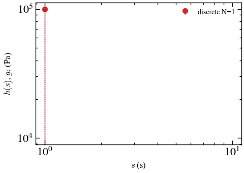

The AIC selects a single mode at the true values (dotted line: true $\tau$ ). The continuous spectrum of a delta function is necessarily broadened by the regularisation and is not shown.

Experimental data: polymer master curve¶

A single frequency sweep covers only a few decades, which limits the range of $s$ that can be resolved: roughly $1/\omega_{\max}\lesssim s\lesssim 1/\omega_{\min}$ . Time–temperature superposition extends this window. The isothermal sweeps from Tutorial 4 are shifted onto a master curve at the reference temperature with CompositeMasterCurve (Lennon et al. [4]), and the spectrum is extracted from the shifted $G'(\omega)$ and $G''(\omega)$ .

from piblin.data import Measurement, OneDimensionalCompositeDataset
from hermes_rheo import read_file
from hermes_rheo.file_readers.trios_rheo_txt import TriosRheoReader
from hermes_rheo.transforms import CompositeMasterCurve

exp = read_file(DATA / "aresg2_trios_frequency_sweep_tts.txt",
                file_reader=TriosRheoReader, create_composite_datasets=True)
mc = CompositeMasterCurve(n_curves=2, y_quantities=["storage modulus", "loss modulus"],
                          x="angular frequency", state="temperature", state_mode="average",
                          vertical_shift=False, sort_states=True, ref_temp_idx=6)(exp)
w, gp = mc.get_mastercurve("storage modulus").datasets[0].data_arrays[:2]
wb, gpp = mc.get_mastercurve("loss modulus").datasets[0].data_arrays[:2]
gpp = np.exp(np.interp(np.log(w), np.log(wb), np.log(gpp)))  # common frequency grid
master = Measurement(datasets=[OneDimensionalCompositeDataset(
    data_arrays=[w, gp * 1e6, gpp * 1e6],  # MPa -> Pa
    data_array_names=["angular frequency", "storage modulus", "loss modulus"],
    data_array_units=["rad/s", "Pa", "Pa"],
    default_independent_name="angular frequency", default_dependent_name="storage modulus")])
print(f"{len(w)} points, {w.min():.1e}-{w.max():.1e} rad/s")

340 points, 1.4e-05-1.1e+10 rad/s

rs = RelaxationSpectrum(domain="frequency")
rs(master)
r = rs.result
print("optimal discrete modes:", len(r.tau))

optimal discrete modes: 18

fig, ax = plt.subplots(figsize=(5.5, 3.8))
plot_relaxation_spectrum(r, ax=ax, show_uncertainty=False)
plt.show()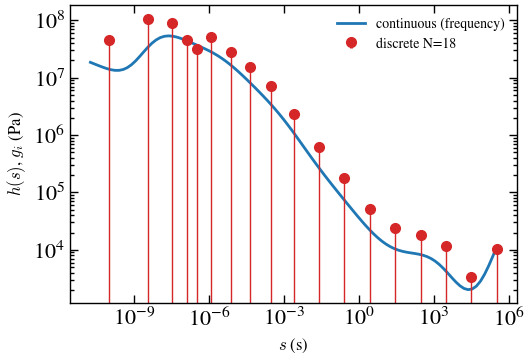

$h(s)$ decreases from the glassy modes ( $s\sim10^{-9}$ –10^-6 s, $h\sim10^{7}$ –10⁸ Pa) through the glass transition to the low-modulus long-time region. The AIC selects 18 discrete modes, roughly one per decade, which is the expected resolution limit for an inversion of this kind. The discrete modes give a compact Maxwell representation that can be used to compute any other linear response (creep compliance, start-up of shear, etc.). The features at both ends of the $s$ axis, including the upturn at the longest times, lie outside the data window $1/\omega_{\max}\lesssim s\lesssim 1/\omega_{\min}$ and should not be interpreted physically.

References¶

Shanbhag, S., pyReSpect: A computer program to extract discrete and continuous spectra from stress relaxation experiments, Macromol. Theory Simul. 28, 1900005 (2019). doi:10.1002/mats.201900005.
Shanbhag, S., Relaxation spectra using nonlinear Tikhonov regularization with a Bayesian criterion, Rheol. Acta 59, 509–520 (2020). doi:10.1007/s00397-020-01212-w.
Takeh, A. & Shanbhag, S., A computer program to extract the continuous and discrete relaxation spectra from dynamic viscoelastic measurements, Appl. Rheol. 23, 24628 (2013). doi:Kroger, Martin et al. (2013).
Lennon, K. R., McKinley, G. H. & Swan, J. W., A data-driven method for automated data superposition with applications in soft matter science, Data-Centric Eng. 4, e13 (2023). doi:Lennon et al. (2023).
Ferry, J. D., Viscoelastic Properties of Polymers, 3rd ed., Wiley (1980).

References¶

Kroger, Martin, Editor Applied Rheology, & editors@appliedrheology.org. (2013). A Computer Program to Extract the Continuous and Discrete Relaxation Spectra from Dynamic Viscoelastic Measurements. 10.3933/APPLRHEOL-23-24628
Lennon, K. R., McKinley, G. H., & Swan, J. W. (2023). A data-driven method for automated data superposition with applications in soft matter science. Data-Centric Engineering, 4. 10.1017/dce.2023.3