Tutorial 9 — Kymographs

A kymograph maps a viscoelastic quantity over two independent variables, for example $\tan\delta(T, \omega)$ over temperature and angular frequency. It shows at a glance where relaxation processes occur and how they move with temperature or time, information that is spread over many curves in conventional sweep plots.

TORCh experiments¶

In a Thermally Optimised Ramped Chirp (TORCh) experiment, OWChirps are applied continuously during a temperature ramp at rate $\dot T$ (Vadillo et al., 2026). Each chirp is time-stamped, so one ramp yields a dense $(T, \omega)$ data set. Here the change of the material is imposed by the ramp rather than by its own kinetics. If the viscoelastic properties are single-valued functions of temperature, the mutation number of Tutorial 6 becomes

(Tutorial 6), so the ramp rate and chirp duration must be chosen to keep $\lvert \mathrm{Mu} \rvert \lesssim 0.15$, especially near thermal transitions where $g$ changes steeply. For low-conductivity samples, the ramp must also be slow compared with heat diffusion through the gap $H$: the diffusion time $\tau_\mathrm{diff} = H^2 \rho C_p / k$, with density $\rho$, heat capacity $C_p$ and thermal conductivity $k$, should be small compared with the mutation time $\lambda_\mathrm{Mu}$, otherwise the sample develops a temperature gradient.

The Kymograph transform¶

Kymograph collects the scattered $(x, y, z)$ points of all measurements and interpolates them onto a regular n_x × n_y grid with scipy.interpolate.griddata; log_y=True interpolates in $\log_{10}\omega$. Each axis is looked up first among the dataset columns and then among the measurement conditions, so either variable can go on either axis; log_x and log_y grid and plot an axis in log scale. The result is a piblin TwoDimensionalDataset with names and units attached.

Temperature–frequency map of $\tan\delta$¶

We use the TORCh ramp of Tutorial 6 (−50 to 150 °C, 10 s chirps). The file already contains the moduli of every chirp; for raw chirp waveforms, prepend OWChirpAnalysis() (Tutorial 3). Peaks in $\tan\delta$ mark relaxation processes such as the glass transition, and their shift to higher frequency with temperature reflects the shift factor $a_T$ (Tutorial 4).

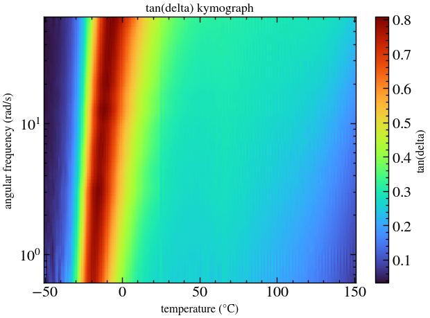
The axes are chosen when the map is built. With frequency on $x$, set log_x=True and log_y=False; the glass transition becomes a band that rises in temperature with frequency.

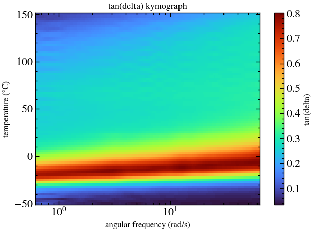
Other quantities and the colour scale¶

Any column can be mapped. The moduli span several decades, so log_z=True uses a logarithmic colour scale; vmin and vmax fix the colour range, for example to round decades or to compare several maps on a common scale.

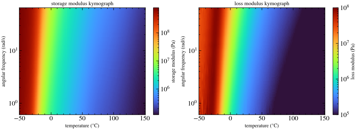
Slices¶

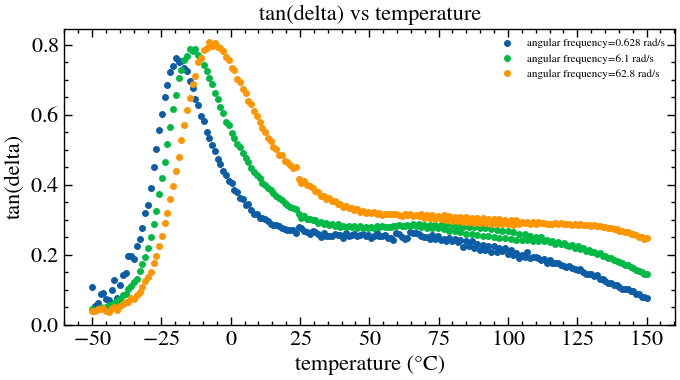
Slices through the grid at fixed $T$ give isothermal frequency sweeps; slices at fixed $\omega$ give isochronal temperature sweeps, as from a dynamic mechanical analysis (DMA) ramp, but both come from a single experiment.

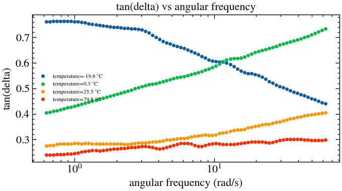
Temperature–frequency map of the mutation number¶

MutationNumber (Tutorial 6) stores temperature and angular frequency with each $\lvert \mathrm{Mu} \rvert$ value, so the same transform maps $\lvert \mathrm{Mu}(T, \omega) \rvert$. Setting vmax=0.15 saturates the colour scale at the quasi-static limit: the brightest regions show where the ramp is closest to the limit.

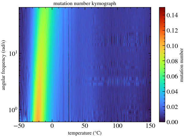
$\lvert \mathrm{Mu} \rvert$ is highest across the glass transition, at all frequencies, and stays well below 0.15 elsewhere. The narrow dark line at 25 °C is the turnaround between the two ramps, where the temperature barely changes between consecutive chirps.

References¶

• Geri, M., Keshavarz, B., Divoux, T., Clasen, C., Curtis, D. J. and McKinley, G. H., Time-Resolved Mechanical Spectroscopy of Soft Materials via Optimally Windowed Chirps, Physical Review X 8, 041042 (2018). DOI: Geri et al. (2018).

• Mours, M. and Winter, H. H., Time-resolved rheometry, Rheologica Acta 33, 385–397 (1994). DOI: Mours & Winter (1994).

• Vadillo, D. C., Perego, A. et al., TORCh: Thermally Optimised Ramped Chirp for time-temperature spectroscopy of polymers, Macromolecules (2026). DOI: Vadillo et al. (2026).