Tutorial 1 — Reading and visualising common rheological datasets - hermes-rheo

This tutorial shows how to load rheometer exports with hermes_rheo and plot them:

A TA Instruments TRIOS .txt export containing a single creep test.
A TRIOS .txt export containing several test types (amplitude sweep, frequency sweep, flow ramp).
An Anton Paar RheoCompass .csv export of a time-temperature superposition (tTS) series of frequency sweeps.

Supported software¶

Software	File type	Reader class
TRIOS	`.txt` (Send To LIMS or To Plain Text (full))	`TriosRheoReader`
RheoCompass	`.csv`	`RheoCompassReader`

All readers are used the same way: read_file takes the file path and, optionally, the reader class. If no reader is given, it is chosen from the file extension (.txt → TriosRheoReader, .csv → RheoCompassReader). For other formats, write a custom reader and reuse the transforms unchanged.

from pathlib import Path

import matplotlib.pyplot as plt
import numpy as np

from hermes_rheo import RheoCompassReader, TriosRheoReader, read_file
from hermes_rheo.visualization import get_unit, use_science_style

use_science_style()  # publication-style Matplotlib settings
DATA = Path("tutorial_data")  # run this notebook from tutorial_notebooks/

1. A file with a single test¶

read_file returns an ExperimentSet when all measurements in the file are of the same kind. Each measurement holds one or more datasets; for a creep step the dataset holds strain as a function of time, so it can be plotted directly. Axis labels and units are read from the file.

creep = read_file(
    DATA / "dhr_trios_creep.txt",
    file_reader=TriosRheoReader,
    create_composite_datasets=True,
)
print(creep)

ExperimentSet
-------------

Summary
-------
Number of Experiments: 1

Varied Conditions
----------------

index	n_rep	method	Data Types	
0	1	Creep - 1	strain(%)=f(time[min]) (483 points)

creep_dataset = creep.measurements[0].datasets[0]
fig, ax = creep_dataset.visualize(marker="o", linewidth=1)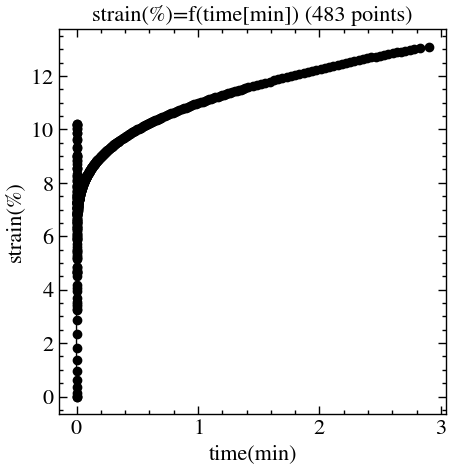

2. A file with several test types¶

A single file can hold different tests in sequence, here an amplitude sweep, a frequency sweep and a flow ramp. They have different axes, so they cannot be grouped in one ExperimentSet. Passing to_experiments=False returns a MeasurementSet instead, where each measurement keeps the axes that suit its test:

amplitude sweep: storage modulus vs. oscillation strain
frequency sweep: storage modulus vs. angular frequency
flow ramp: viscosity vs. shear rate

tests = read_file(
    DATA / "dhr_trios_multi_technique.txt",
    file_reader=TriosRheoReader,
    create_composite_datasets=True,
    to_experiments=False,
)

for measurement in tests.measurements:
    dataset = measurement.datasets[0]
    print(
        f"{measurement.conditions['method']:<22}"
        f"{dataset.dependent_variable_name} vs. {dataset.independent_variable_name}"
    )

Amplitude sweep - 1   storage modulus vs. oscillation strain (cmd)
Frequency sweep - 2   storage modulus vs. angular frequency
Flow ramp - 3         viscosity vs. shear rate

Selecting and plotting a measurement¶

Measurements are indexed in the order they appear in the file. visualize() plots a dataset on its default axes and returns the Matplotlib figure and axes for further formatting.

amplitude_sweep, frequency_sweep, flow_ramp = (m.datasets[0] for m in tests.measurements)

fig, ax = amplitude_sweep.visualize(marker="o", linewidth=1, color="red")
ax.set_xscale("log")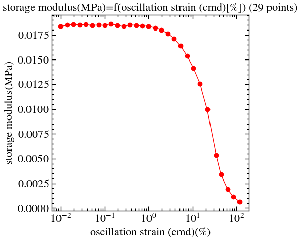

fig, ax = frequency_sweep.visualize(marker="s", linewidth=1, color="black")
ax.set_xscale("log")
ax.set_yscale("log")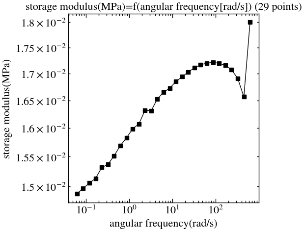

fig, ax = flow_ramp.visualize(marker="^", linewidth=1, color="green")
ax.set_xscale("log")
ax.set_yscale("log")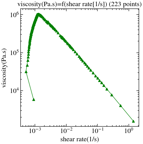

Switching axes and accessing the data¶

Every dataset stores all the columns of its test. switch_coordinates() changes the plotted pair, and the arrays are available as x_values (independent variable) and y_values (dependent variable).

frequency_sweep.switch_coordinates("angular frequency", "complex viscosity")
fig, ax = frequency_sweep.visualize(marker="s", linewidth=1, color="black")
ax.set_xscale("log")
ax.set_yscale("log")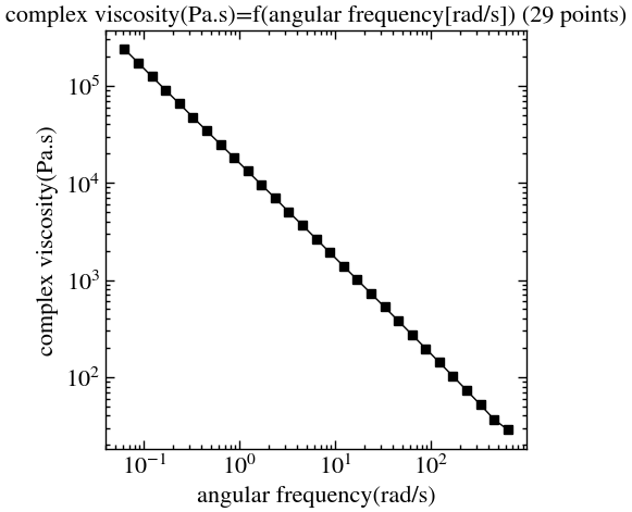

print(f"{frequency_sweep.independent_variable_name}: {frequency_sweep.x_values[:3]}")
print(f"{frequency_sweep.dependent_variable_name}: {frequency_sweep.y_values[:3]}")

angular frequency: [+628.3185 +452.1964 +325.4363]
complex viscosity: [+28.7017 +36.6608 +51.9980]

3. A RheoCompass file¶

RheoCompassReader is used exactly like TriosRheoReader. The file below is a tTS series: isothermal frequency sweeps measured at different temperatures, one measurement per interval. Plotting a few of them shows how the moduli shift with temperature; visualize(axes=...) draws each sweep on a shared axis and labels it from the dataset. Tutorial 4 builds the master curve from this kind of data.

experiment = read_file(
    DATA / "mcr702e_rheocompass_tts.csv",
    file_reader=RheoCompassReader,
    create_composite_datasets=True,
)

isotherms = experiment.measurements[4::6]  # every 6th temperature, from 80 °C down
colors = plt.cm.coolwarm(np.linspace(1, 0, len(isotherms)))  # red = hot, blue = cold

fig, (ax_storage, ax_loss) = plt.subplots(1, 2, figsize=(10, 4))
for measurement, color in zip(isotherms, colors):
    sweep = measurement.datasets[0]
    temperature = sweep.data_arrays[sweep.data_array_names.index("temperature")].mean()
    label = f"T = {temperature:.0f} {get_unit(sweep, 'temperature')}"
    sweep.visualize(axes=ax_storage, marker="s", linestyle="none", color=color, label=label)
    sweep.switch_coordinates("angular frequency", "loss modulus")
    sweep.visualize(axes=ax_loss, marker="o", linestyle="none", color=color, mfc="none")

for ax in (ax_storage, ax_loss):
    ax.set_xscale("log")
    ax.set_yscale("log")
handles, labels = ax_storage.get_legend_handles_labels()
ax_loss.legend(handles[::-1], labels[::-1], loc="center left", bbox_to_anchor=(1.02, 0.5))  # cold on top
fig.tight_layout()
plt.show()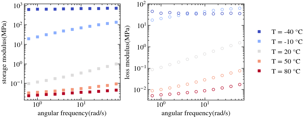

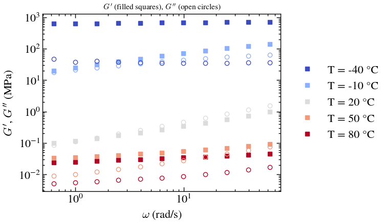
Customising the plot¶

visualize() returns standard Matplotlib objects, so any element can be changed afterwards. Below, G′ and G″ share one axis, and the default labels are replaced by symbols while the units are still read from the dataset.

fig, ax = plt.subplots(figsize=(6, 4.5))
for measurement, color in zip(isotherms, colors):
    sweep = measurement.datasets[0]
    temperature = sweep.data_arrays[sweep.data_array_names.index("temperature")].mean()
    label = f"T = {temperature:.0f} {get_unit(sweep, 'temperature')}"
    sweep.switch_coordinates("angular frequency", "storage modulus")
    sweep.visualize(axes=ax, marker="s", linestyle="none", color=color, label=label)
    sweep.switch_coordinates("angular frequency", "loss modulus")
    sweep.visualize(axes=ax, marker="o", linestyle="none", color=color, mfc="none", label="_")

ax.set_xscale("log")
ax.set_yscale("log")
ax.set_xlabel(rf"$\omega$ ({get_unit(sweep, 'angular frequency')})")
ax.set_ylabel(rf"$G'$, $G''$ ({get_unit(sweep, 'storage modulus')})")
ax.set_title(r"$G'$ (filled squares), $G''$ (open circles)", fontsize=11)
handles, labels = ax.get_legend_handles_labels()
ax.legend(handles[::-1], labels[::-1], loc="center left", bbox_to_anchor=(1.02, 0.5))
plt.show()