Tutorial 11 — Rheological model fitting - hermes-rheo

FitModel fits constitutive models to small-amplitude oscillatory shear (SAOS) moduli $G'(\omega)$ , $G''(\omega)$ or to a relaxation modulus $G(t)$ . It accepts a single sweep, one temperature of a time–temperature superposition (TTS) series, or a master curve. Two engines are available:

the built-in generalized Maxwell (Prony series) model, and
the classical and fractional models of pyRheo (Miranda-Valdez et al., 2025), an optional dependency.

Each fit returns a piblin Measurement holding the data, the fitted curves and, in details, the parameters and goodness of fit. The data are a discrete frequency sweep of a polymer melt at 49 °C.

pyRheo draws random initial guesses from NumPy’s global generator, so the notebook seeds it for reproducible results.

import contextlib
import io
import warnings
from pathlib import Path

import matplotlib.pyplot as plt
import numpy as np

from hermes_rheo import read_file
from hermes_rheo.file_readers.trios_rheo_txt import TriosRheoReader
from hermes_rheo.transforms.fit_model import FitModel
from hermes_rheo.transforms.frequency_to_time import FrequencyToTime
from hermes_rheo.visualization import use_science_style

use_science_style()
warnings.filterwarnings("ignore")  # pyRheo emits numerical warnings during optimisation
np.random.seed(0)  # pyRheo draws random initial guesses; seed for reproducibility

DATA = Path("tutorial_data")  # run from tutorial_notebooks/

experiment = read_file(
    DATA / "dhr30_trios_owchirp_vs_frequency_sweep.txt",
    file_reader=TriosRheoReader,
    create_composite_datasets=True,
)
# Each measurement is one OWChirp spectrum recorded during a temperature ramp;
# pick the one closest to 49 °C.
temperatures = np.array([
    m.datasets[0].data_arrays[m.datasets[0].data_array_names.index("temperature")].mean()
    for m in experiment.measurements
])
sweep = experiment.measurements[int(np.argmin(np.abs(temperatures - 49.0)))]

SAOS: classical and generalized Maxwell¶

A Maxwell element, a spring of modulus $G$ in series with a dashpot of viscosity $\eta$ , relaxes with a single time $\tau = \eta/G$ :

G'(\omega) = G\,\frac{(\omega\tau)^2}{1 + (\omega\tau)^2}, \qquad G''(\omega) = G\,\frac{\omega\tau}{1 + (\omega\tau)^2}.

(1)

The generalized Maxwell model places $N$ such elements in parallel, giving the Prony series $G(t) = G_e + \sum_i g_i\, e^{-t/\tau_i}$ and

G'(\omega) = G_e + \sum_{i=1}^{N} g_i\,\frac{(\omega\tau_i)^2}{1 + (\omega\tau_i)^2}, \qquad G''(\omega) = \sum_{i=1}^{N} g_i\,\frac{\omega\tau_i}{1 + (\omega\tau_i)^2}.

(2)

With mode="nnls" (default), the $\tau_i$ are fixed on a logarithmic grid spanning the data and the moduli $g_i \ge 0$ are found by non-negative least squares, which is fast and needs no initial guesses. The equilibrium modulus $G_e$ is included with equilibrium_modulus=True.

def fit(transform, target):
    """Apply a FitModel transform, silencing the optimiser's progress prints."""
    with contextlib.redirect_stdout(io.StringIO()):
        return transform(target)


fits = {
    "Maxwell": FitModel(model_name="Maxwell"),
    "4-mode Maxwell": FitModel(model="custom", model_name="MultiModeMaxwell", n_modes=4),
}
results = {name: fit(f, sweep) for name, f in fits.items()}
for name, r in results.items():
    print(name, r.details["parameters"])

Maxwell {'G_s': 75030.68610525543, 'eta_s': 13741.92891933592}
4-mode Maxwell {'G_modes': [116393.8358305254, 27882.31360585928, 0.0, 38770.13968926155], 'tau_modes': [0.01591549459100615, 0.07387318085377693, 0.3428889261499121, 1.591549386630056], 'equilibrium_modulus': 0.0}

SAOS: fractional model¶

Many soft materials relax as a power law over decades of frequency, which requires many Maxwell modes. A spring-pot (Scott Blair element) interpolates between a spring and a dashpot,

\sigma(t) = V\,\frac{\mathrm{d}^{\alpha}\gamma(t)}{\mathrm{d}t^{\alpha}}, \qquad G^{*}(\omega) = V\,(i\omega)^{\alpha}, \qquad 0 \le \alpha \le 1,

(3)

so $\alpha = 0$ is a spring and $\alpha = 1$ a dashpot, and its phase angle $\delta = \alpha\pi/2$ is independent of frequency. Combining spring-pots gives compact models with few parameters (Bonfanti et al., 2020; Song et al., 2023). The fractional Kelvin–Voigt model places two spring-pots in parallel,

G^{*}(\omega) = V\,(i\omega)^{\alpha} + G\,(i\omega)^{\beta},

(4)

and captures the two power-law regimes of this sweep with four parameters. The plot compares the three models: one Maxwell mode cannot describe a broad spectrum, four modes approximate it with visible ripples, and the fractional model follows the data closely.

fits["Fractional Kelvin–Voigt"] = FitModel(model_name="FractionalKelvinVoigt")
results["Fractional Kelvin–Voigt"] = fit(fits["Fractional Kelvin–Voigt"], sweep)
print("Fractional Kelvin–Voigt", results["Fractional Kelvin–Voigt"].details["parameters"])

Fractional Kelvin–Voigt {'G': 3178.418976149676, 'V': 42725.90973579788, 'alpha': 0.17453102613238186, 'beta': 0.7293643795406608}

fig, axes = plt.subplots(1, 2, figsize=(10, 4), sharex=True)
for ax, y in zip(axes, ("storage modulus", "loss modulus")):
    for i, (name, r) in enumerate(results.items()):
        ds = r.datasets[0]
        arr, unit = dict(zip(ds.data_array_names, ds.data_arrays)), dict(zip(ds.data_array_names, ds.data_array_units))
        x = "angular frequency"
        if i == 0:
            ax.loglog(arr[x], arr[y], "ko", ms=3, label="data")
        ax.loglog(arr[x], arr[f"fitted {y}"], label=name)
    ax.set(xlabel=f"{x} [{unit[x]}]", ylabel=f"{y} [{unit[y]}]")
    ax.legend(frameon=False, fontsize=8)
plt.tight_layout()
plt.show()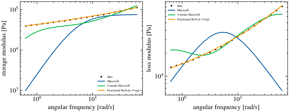

Relaxation domain¶

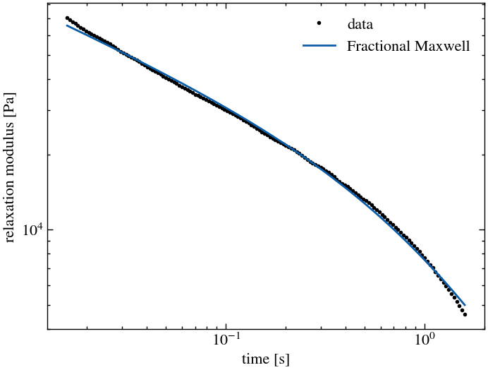
FrequencyToTime reconstructs $G(t)$ from the sweep (Tutorial 12), and FitModel(domain="relaxation") fits it directly; the multi-mode Maxwell model is available only for SAOS data. The fractional Maxwell model places two spring-pots in series,

G(t) = G\,t^{-\beta}\,E_{\alpha-\beta,\,1-\beta}\!\left(-\frac{G}{V}\,t^{\alpha-\beta}\right),

(5)

where $E_{a,b}$ is the two-parameter Mittag-Leffler function. It describes a power-law decay $G(t) \sim t^{-\beta}$ at short times followed by faster relaxation at long times. Here minimization_algorithm="Powell" gives a more robust optimum than the default L-BFGS-B.

relaxation = FrequencyToTime(n_time_points=150)(sweep)
relax_fit = FitModel(domain="relaxation", model_name="FractionalMaxwell",
                     minimization_algorithm="Powell")
r = fit(relax_fit, relaxation)
print("Fractional Maxwell", r.details["parameters"])

ds = r.datasets[0]
arr, unit = dict(zip(ds.data_array_names, ds.data_arrays)), dict(zip(ds.data_array_names, ds.data_array_units))
plt.loglog(arr["time"], arr["relaxation modulus"], "ko", ms=3, label="data")
plt.loglog(arr["time"], arr["fitted relaxation modulus"], label="Fractional Maxwell")
plt.xlabel(f"time [{unit['time']}]")
plt.ylabel(f"relaxation modulus [{unit['relaxation modulus']}]")
plt.legend(frameon=False)
plt.show()

Fractional Maxwell {'G': 22397.70845533997, 'V': 52045.80882040109, 'alpha': 0.9899999996740758, 'beta': 0.3490522618921849}

References¶

Bonfanti, A., Kaplan, J. L., Charras, G. and Kabla, A., Fractional viscoelastic models for power-law materials, Soft Matter 16, 6002–6020 (2020). DOI: 10.1039/d0sm00354a.
Song, J., Holten-Andersen, N. and McKinley, G. H., Non-Maxwellian viscoelastic stress relaxations in soft matter, Soft Matter 19, 7885–7906 (2023). DOI: 10.1039/d3sm00736g.
Miranda-Valdez, I. Y., Niinistö, J., Mäkinen, T., Lejon, J., Koivisto, J. and Alava, M. J., pyRheo: an open-source Python package for complex rheology, Digital Discovery 4, 1075–1082 (2025). DOI: 10.1039/d5dd00021a.