Tutorial 12 — Relaxation modulus from SAOS data - hermes-rheo

The relaxation modulus $G(t)$ and the dynamic moduli $G'(\omega)$ , $G''(\omega)$ carry the same linear viscoelastic information, but converting between them normally requires fitting a model (for example a Prony series) or evaluating a Fourier integral numerically on finite, noisy data. FrequencyToTime implements i-Rheo-Tempo (Ramírez and Tassieri, 2026), a model-free and quadrature-free reconstruction.

From moduli to complex viscosity¶

With $G^{*}(\omega) = G'(\omega) + i\,G''(\omega)$ , the complex viscosity is

\eta^{*}(\omega) = \frac{G^{*}(\omega)}{i\omega} = \eta'(\omega) - i\,\eta''(\omega), \qquad \eta'(\omega) = \frac{G''(\omega)}{\omega}, \qquad \eta''(\omega) = \frac{G'(\omega)}{\omega}.

(1)

$G(t)$ follows from either component by a Fourier transform,

G_{\eta'}(t) = \frac{2}{\pi}\int_0^{\infty} \eta'(\omega)\cos(\omega t)\,\mathrm{d}\omega, \qquad G_{\eta''}(t) = \frac{2}{\pi}\int_0^{\infty} \eta''(\omega)\sin(\omega t)\,\mathrm{d}\omega + \frac{2}{\pi}\frac{\eta''(0)}{t}.

(2)

For viscoelastic liquids $\eta''(0) = 0$ (default enforce_eta2_zero=True).

Interval-slope reconstruction¶

i-Rheo-Tempo interpolates $\eta'$ and $\eta''$ between data points and treats them as piecewise linear on intervals $[\omega_{L,k}, \omega_{R,k}]$ with slopes $a_{1,k}$ and $a_{2,k}$ . The integrals then have closed forms,

G_{\eta'}(t) = \frac{2}{\pi t^{2}}\sum_k \left[\cos(\omega_{R,k}t) - \cos(\omega_{L,k}t)\right] a_{1,k},

(3)

G_{\eta''}(t) = \frac{2}{\pi t^{2}}\sum_k \left[\sin(\omega_{R,k}t) - \sin(\omega_{L,k}t)\right] a_{2,k} + \frac{2}{\pi}\frac{\eta''(0)}{t},

(4)

so no quadrature is needed. Before the sum, the spectrum is anchored at low frequency by a log–log polynomial fit for $\eta'(0)$ and extended at high frequency by a polynomial extrapolation.

The transform returns a time-domain dataset with G_from_eta1 ( $G_{\eta'}$ ) and G_from_eta2 ( $G_{\eta''}$ ), followed by the original datasets. The full result, with the processed grid and diagnostics, is stored in details["frequency_to_time_result"]. Inputs must be in SI units (rad/s, Pa). The two estimates should agree within the reliable time window, roughly $1/\omega_\mathrm{max} \lesssim t \lesssim 1/\omega_\mathrm{min}$ ; disagreement flags limited bandwidth or interpolation artefacts at its edges.

import warnings
from pathlib import Path

import matplotlib.pyplot as plt
import numpy as np

from hermes_rheo.lve_models import MaxwellModel, Protocols
from hermes_rheo.transforms import FrequencyToTime
from hermes_rheo.visualization import use_science_style

use_science_style()
warnings.filterwarnings("ignore")  # master-curve optimiser convergence notices
DATA = Path("tutorial_data")

Validation: single-mode Maxwell model¶

A single Maxwell element with $G = 10^5$ Pa and $\tau = 1$ s has the moduli

G'(\omega) = G\,\frac{(\omega\tau)^2}{1 + (\omega\tau)^2}, \qquad G''(\omega) = G\,\frac{\omega\tau}{1 + (\omega\tau)^2},

(5)

and the exact relaxation modulus $G(t) = G\,e^{-t/\tau}$ . Protocols.saos evaluates the moduli on 60 frequencies from 10^-2 to 10² rad/s, and the reconstruction is compared with the exact result.

G0, tau = 1e5, 1.0
saos = Protocols.saos(MaxwellModel(G=G0, tau=tau), np.geomspace(1e-2, 1e2, 60))
out = FrequencyToTime()(saos)
t, g1, g2 = out.datasets[0].data_arrays
sel = (t > 0.02) & (t < 5)
print(f"max relative error vs analytic G(t), 0.02-5 s: eta1 {np.max(abs(g1[sel]/(G0*np.exp(-t[sel]/tau))-1)):.1e}, "
      f"eta2 {np.max(abs(g2[sel]/(G0*np.exp(-t[sel]/tau))-1)):.1e}")

max relative error vs analytic G(t), 0.02-5 s: eta1 1.1e-04, eta2 1.9e-03

fig, ax = plt.subplots(figsize=(5, 3.6))
ax.loglog(t, G0 * np.exp(-t / tau), "k-", label=r"analytic $Ge^{-t/\tau}$")
ax.loglog(t, g1, "o", ms=3, label=r"from $\eta'$")
ax.loglog(t, g2, "s", ms=3, mfc="none", label=r"from $\eta''$")
ax.set(xlabel="time (s)", ylabel="G(t) (Pa)", ylim=(1e0, 2e5)); ax.legend()
plt.show()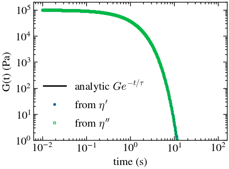

The reconstruction follows the exponential decay over the covered window; deviations appear only at times outside the measured frequency range ( $\sim 1/\omega_\mathrm{max}$ to $\sim 1/\omega_\mathrm{min}$ ).

Experimental data: polymer melt, time–temperature superposition¶

A single frequency sweep spans two or three decades, which limits $G(t)$ to a similarly narrow window. Time–temperature superposition (Tutorial 4) extends the spectrum: CompositeMasterCurve shifts $G'$ and $G''$ jointly onto one master curve at 20 °C (Lennon et al., 2023), covering about 15 decades of reduced frequency $a_T\,\omega$ . Reconstructing $G(t)$ from it gives the relaxation modulus over a correspondingly broad time window.

from piblin.data import Measurement, OneDimensionalCompositeDataset
from hermes_rheo import read_file
from hermes_rheo.file_readers.trios_rheo_txt import TriosRheoReader
from hermes_rheo.transforms import CompositeMasterCurve

exp = read_file(DATA / "aresg2_trios_frequency_sweep_tts.txt",
                file_reader=TriosRheoReader, create_composite_datasets=True)
mc = CompositeMasterCurve(n_curves=2, y_quantities=["storage modulus", "loss modulus"],
                          x="angular frequency", state="temperature", state_mode="average",
                          vertical_shift=False, sort_states=True, ref_temp_idx=6)(exp)
w, gp = mc.get_mastercurve("storage modulus").datasets[0].data_arrays[:2]
wb, gpp = mc.get_mastercurve("loss modulus").datasets[0].data_arrays[:2]
gpp = np.exp(np.interp(np.log(w), np.log(wb), np.log(gpp)))  # common frequency grid
master = Measurement(datasets=[OneDimensionalCompositeDataset(
    data_arrays=[w, gp * 1e6, gpp * 1e6],  # MPa -> Pa
    data_array_names=["angular frequency", "storage modulus", "loss modulus"],
    data_array_units=["rad/s", "Pa", "Pa"],
    default_independent_name="angular frequency", default_dependent_name="storage modulus")])
print(f"{len(w)} points, {w.min():.1e}-{w.max():.1e} rad/s")

340 points, 1.4e-05-1.1e+10 rad/s

ft = FrequencyToTime()
res = ft(master)
t, g1, g2 = res.datasets[0].data_arrays
fig, (a, b) = plt.subplots(1, 2, figsize=(9, 3.6))
a.loglog(w, gp * 1e6, "o", ms=2, label="G'"); a.loglog(w, gpp * 1e6, "s", ms=2, label="G''")
a.set(xlabel="angular frequency (rad/s)", ylabel="modulus (Pa)"); a.legend()
b.loglog(t, g1, "-", label=r"from $\eta'$")
b.set(xlabel="time (s)", ylabel="G(t) (Pa)"); b.legend()
plt.tight_layout(); plt.show()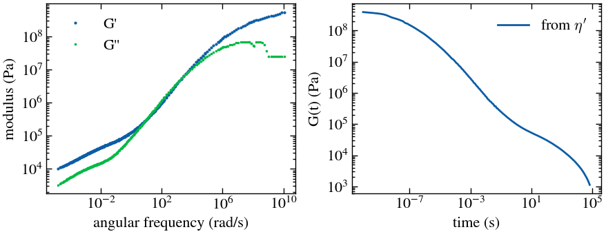

$G(t)$ decays from the glassy short-time response ( $\sim 10^8$ Pa) through the glass transition to a rubbery shoulder around 10⁴–10⁵ Pa. Because $G' > G''$ even at the lowest shifted frequency, the master curve does not reach the terminal regime, and the drop beyond $\sim 10^{4}$ s reflects the end of the data window rather than terminal flow. The $\eta'$ estimate is the more robust one for noisy master curves; the $\eta''$ estimate oscillates at short times and is not shown.

Further options control the low-frequency anchor (lf_poly_order, lf_fit_decades), the high-frequency extension (hf_poly_order, hf_fit_decades, hf_ext_decades), the interpolant (interpolation_method="spline", "pchip" or "csaps"), and an optional single-mode Maxwell terminal tail (fit_maxwell_tail=True).

References¶

Ramírez, J. and Tassieri, M., i-Rheo-Tempo: A model-free, quadrature-free reconstruction of the shear relaxation modulus from complex viscosity, Journal of Rheology 70, 1089–1104 (2026). DOI: 10.1122/8.0001232. Reference implementation: University of Glasgow Research Data, Tassieri & Ramírez (2026).
Lennon, K. R., McKinley, G. H. and Swan, J. W., A data-driven method for automated data superposition with applications in soft matter science, Data-Centric Engineering 4, e13 (2023). DOI: Lennon et al. (2023).