For thermorheologically simple materials, a change in temperature rescales all relaxation times by the same factor . Spectra measured at different temperatures therefore superpose on a single master curve at a reference temperature after a horizontal shift along the frequency axis,
which extends the accessible frequency window by several decades.
Automated superposition
AutomatedMasterCurve estimates the shifts with the method of Lennon et al.
(2023). Each data set is interpolated by a Gaussian process that includes an
estimate of interpolation uncertainty, and the shift between neighbouring data
sets is the one that maximizes the posterior probability of their overlap. The
pairwise shifts are accumulated relative to the reference state, and each
is returned with its uncertainty. No functional form of is
assumed.
Shift-factor models
The temperature dependence of is described afterwards. Above the glass transition, the Williams–Landel–Ferry (WLF) equation (Williams et al., 1955)
usually applies, while the Arrhenius equation
with in kelvin and activation energy , suits melts well above
and thermally activated processes. Both are available in ShiftFactorModel.
The same pressure sensitive adhesive (PSA) was measured with a conventional frequency sweep and
with OWChirp (Geri et al., 2018; Perego et al., 2025); OWChirpAnalysis
first converts the chirp signals to , and (Tutorial 3).
import warnings
from pathlib import Path

import matplotlib.pyplot as plt

from hermes_rheo import read_file
from hermes_rheo.file_readers.trios_rheo_txt import TriosRheoReader
from hermes_rheo.transforms.automated_mastercurve import AutomatedMasterCurve, CompositeMasterCurve
from hermes_rheo.transforms.owchirp_analysis import OWChirpAnalysis
from hermes_rheo.transforms.shift_factor_models import ShiftFactorModel
from hermes_rheo.visualization import axis_label, plot_master_curve, plot_shift_factors, use_science_style

use_science_style()
warnings.filterwarnings("ignore")  # scikit-learn / SciPy convergence notices
DATA = Path("tutorial_data")
T_REF = 20  # reference temperature, °C
Master curves
Both data sets are superposed on the storage modulus .
state_mode="average" assigns each frequency sweep or chirp the mean of its
recorded temperature, which absorbs small drifts during the measurement.
change_ref moves the reference to the state closest to and
rescales all shift factors so that .
settings = dict(state="temperature", state_mode="average",
                x="angular frequency", y="storage modulus")

sweep = read_file(DATA / "aresg2_trios_frequency_sweep_tts.txt",
                  file_reader=TriosRheoReader, create_composite_datasets=True)
chirp = OWChirpAnalysis()(read_file(DATA / "aresg2_trios_owchirp_tts.txt",
                                    file_reader=TriosRheoReader, create_composite_datasets=True))

mc_sweep = AutomatedMasterCurve(**settings)(sweep)
mc_chirp = AutomatedMasterCurve(**settings)(chirp)
for mc in (mc_sweep, mc_chirp):
    mc.change_ref(min(mc.states, key=lambda T: abs(T - T_REF)))
fig, axes = plot_master_curve(mc_sweep)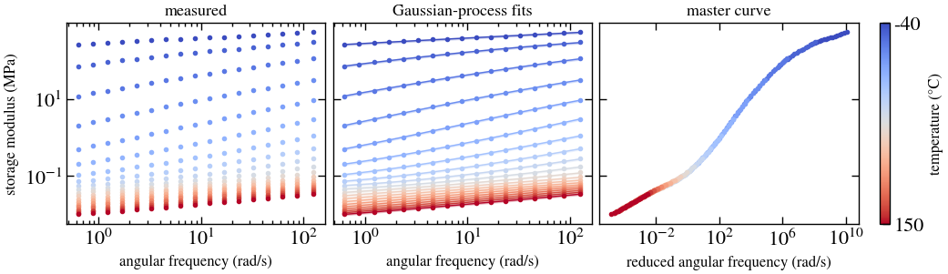
plot_master_curve shows the frequency-sweep data before shifting, the
Gaussian-process interpolants used to find the shifts (mean ± one standard
deviation), and the master curve against the reduced frequency .
The colour bar gives the temperature range. Twenty isotherms between -40 and
150 °C, each covering little more than two decades, combine into a master
curve spanning about fourteen decades, from the glassy plateau at high
to the low-modulus region at low .
Shift factors
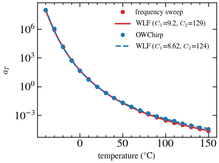
ShiftFactorModel(model="WLF") fits and to the shift factors of
each master curve; use
model="Arrhenius" for the activation-energy form. Agreement of the two
fits confirms that OWChirp recovers the same temperature dependence as the
frequency sweep.
wlf_sweep = ShiftFactorModel(model="WLF")(mc_sweep)
wlf_chirp = ShiftFactorModel(model="WLF")(mc_chirp)
wlf_sweep.print_parameters()
wlf_chirp.print_parameters()

fig, ax = plot_shift_factors(wlf_sweep, data_label="frequency sweep", figsize=(4.5, 3.4),
                             color="tab:red", data_color="tab:red")
plot_shift_factors(wlf_chirp, ax=ax, data_label="OWChirp", linestyle="--",
                   color="tab:blue", data_color="tab:blue");
WLF: C1 = 9.203, C2 = 128.8, Tref = 20.01
WLF: C1 = 8.625, C2 = 123.6, Tref = 19.99
Frequency sweep and OWChirp
The two master curves are compared directly. The units are read from the
data: TRIOS exports the frequency-sweep moduli in MPa, while OWChirpAnalysis
returns Pa. piblin’s change_dependent_variable_data_unit converts the
frequency-sweep curve before plotting.
TO_PA = {"Pa": 1.0, "kPa": 1e3, "MPa": 1e6} # Conversion factors to Pascal (Pa)

fig, ax = plt.subplots(figsize=(4.5, 3.4))
for mc, color, label in ((mc_sweep, "tab:red", "frequency sweep"), (mc_chirp, "tab:blue", "OWChirp")):
    curve = mc.datasets[0]
    curve.change_dependent_variable_data_unit(TO_PA[curve.y_unit], "Pa")
    ax.loglog(curve.x_values, curve.y_values, "o", ms=3, color=color, label=label)
ax.set(xlabel=axis_label(curve, curve.x_name, text=r"$a_T\,\omega$"),
       ylabel=axis_label(curve, curve.y_name, text="$G'$"))
ax.legend(loc="upper left", fontsize=12);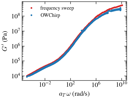
, and from the frequency sweep
CompositeMasterCurve builds one master curve per quantity, each with its own
Gaussian-process shift. Since is independent of any
vertical (modulus) shift, its master curve is a useful check of
thermorheological simplicity.
composite = CompositeMasterCurve(n_curves=3, y_quantities=["storage modulus", "loss modulus", "tan(delta)"],
                                 state="temperature", x="angular frequency")(sweep)
for mc in composite.measurements:
    mc.change_ref(min(mc.states, key=lambda T: abs(T - T_REF)))
gp, gpp, tan_delta = (mc.datasets[0] for mc in composite.measurements)

fig, ax = plt.subplots(figsize=(5, 3.6))
ax_tan = ax.twinx()
ax.loglog(gp.x_values, gp.y_values, "o", ms=3, color="tab:blue", label="$G'$")
ax.loglog(gpp.x_values, gpp.y_values, "o", ms=3, color="tab:green", label="$G''$")
ax_tan.semilogx(tan_delta.x_values, tan_delta.y_values, "o", ms=3, color="tab:red", label=r"$\tan\delta$")

ax.set(xlabel=axis_label(gp, gp.x_name, text=r"$a_T\,\omega$"),
       ylabel=axis_label(gp, gp.y_name, text="$G'$, $G''$"))
ax.tick_params(which="both", right=False)
ax_tan.set_ylabel(r"$\tan\delta$", color="tab:red")
ax_tan.tick_params(axis="y", which="both", colors="tab:red")
handles = ax.get_legend_handles_labels()[0] + ax_tan.get_legend_handles_labels()[0]
ax.legend(handles=handles, loc="upper left");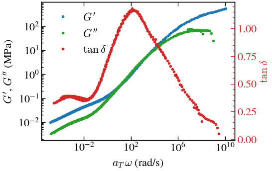
The OWChirp data were decimated by a factor of 4 (sampling rate from 500 pt/s to 125 pt/s, every 4th point kept) to reduce file size; the full-resolution files are available on request from Alessandro Perego (aperego@mmm.com).
References
Lennon, K. R., McKinley, G. H., Swan, J. W., Data-Centric Engineering 2023, 4, e13. Lennon et al. (2023)
Geri, M., Keshavarz, B., McKinley, G. H., Swan, J. W., Phys. Rev. X 2018, 8, 041042. Geri et al. (2018)
Perego, A. et al., Rheologica Acta 2025. Perego et al. (2025)
Williams, M. L., Landel, R. F., Ferry, J. D., J. Am. Chem. Soc. 1955, 77, 3701. Williams et al. (1955)
- Lennon, K. R., McKinley, G. H., & Swan, J. W. (2023). A data-driven method for automated data superposition with applications in soft matter science. Data-Centric Engineering, 4. 10.1017/dce.2023.3
- Geri, M., Keshavarz, B., Divoux, T., Clasen, C., Curtis, D. J., & McKinley, G. H. (2018). Time-Resolved Mechanical Spectroscopy of Soft Materials via Optimally Windowed Chirps. Physical Review X, 8(4). 10.1103/physrevx.8.041042
- Perego, A., Vadillo, D. C., Mills, M. J. L., Das, M., & McKinley FRS, G. H. (2025). Evaluation of optimally windowed chirp signals in industrial rheological measurements: method development and data processing. Rheologica Acta, 64(8), 391–406. 10.1007/s00397-025-01511-0
- Williams, M. L., Landel, R. F., & Ferry, J. D. (1955). The Temperature Dependence of Relaxation Mechanisms in Amorphous Polymers and Other Glass-forming Liquids. Journal of the American Chemical Society, 77(14), 3701–3707. 10.1021/ja01619a008